Bibliography

1

PAPI: Performance Application Programming Interface.
http://icl.cs.utk.edu/projects/papi/.

2

PCL -- The Performance Counter Library.
http://www.fz-juelich.de/zam/PCL/.

3

Sameer Shende, Allen D. Malony, Craig Rasmussen, and Matt Sottile.
A Performance Interface for Component-Based Applications.
In Proceedings of International Workshop on Performance Modeling, Evaluation and Optimization, International Parallel and Distributed Processing Symposium, 2003.

4

Darren J. Kerbyson, Henry J. Alme, Adolfy Hoisie, Fabrizio Petrini, Harvey J. Wasserman, and Michael L. Gittings.
Predictive performance and scalability modeling of a large-scale application.
In Proceedings of Supercomputing, 2001.
Distributed via CD-ROM.

5

Darren J. Kerbyson, Harvey J Wasserman, and Adolfy Hoisie.
Exploring advanced architectures using performance prediction.
In International Workshop on Innovative Architectures, pages 27-40. IEEE Computer Society Press, 2002.

6

R. Englander and M. Loukides.
Developing Java Beans (Java Series).
O'Reilly and Associates, 1997.
http://www.java.sun.com/products/javabeans.

7

CORBA Component model webpage.
http://www.omg.com.
Accessed July 2002.

8

B. A. Allan, R. C. Armstrong, A. P. Wolfe, J. Ray, D. E. Bernholdt, and J. A. Kohl.
The CCA core specifications in a distributed memory SPMD framework.
Concurrency: Practice and Experience, 14:323-345, 2002.
Also at http://www.cca-forum.org/ccafe03a/index.html.

9

Rob Armstrong, Dennis Gannon, Al Geist, Katarzyna Keahey, Scott R. Kohn, Lois McInnes, Steve R. Parker, and Brent A. Smolinski.
Toward a Common Component Architecture for High-Performance Scientific Computing.
In Proceedings of High Performance Distributed Computing Symposium, 1999.

10

Sophia Lefantzi, Jaideep Ray, and Habib N. Najm.
Using the Common Component Architecture to Design High Performance Scientific Simulation Codes.
In Proceedings of International Parallel and Distributed Processing Symposium, 2003.

11

Sameer Shende, Allen D. Malony, and Robert Ansell-Bell.
Instrumentation and measurement strategies for flexible and portable empirical performance evaluation.
In Proceedings of the International Conference on Parallel and Distributed Processing Techniques and Applications, PDPTA '2001, pages 1150-1156. CSREA, June 2001.

12

Jim Maloney.
Distributed COM Application Development Using Visual C++ 6.0.
Prentice Hall PTR, 1999.
ISBN 0130848743.

13

Adrian Mos and John Murphy.
Performance Monitoring of Java Component-oriented Distributed Applications.
In IEEE 9th International Conference on Software, Telecommunications and Computer Networks - SoftCOM, 2001.

14

Baskar Sridharan, Balakrishnan Dasarathy, and Aditaya Mathur.
On Building Non-Intrusive Performance Instrumentation Blocks for CORBA-based Distributed Systems.
In 4th IEEE International Computer Performance and Depenability Symposium, March 2000.

15

Baskar Sridharan, Sambhrama Mundkur, and Aditaya Mathur.
Non-intrusive Testing, Monitoring and Control of Distributed CORBA Objects.
In TOOLS Europe 2000, June 2000.

16

Nathalie Furmento, Anthony Mayer, Stepen McGough, Steven Newhouse, Tony Field, and John Darlington.
Optimisation of Component-based Applications within a Grid Environment.
In Proceedings of Supercomputing, 2001.
Distributed via CD-ROM.

17

Nathalie Furmento, Anthony Mayer, Stepen McGough, Steven Newhouse, Tony Field, and John Darlington.
ICENI: Optimisation of Component Applications within a Grid Environment.
Parallel Computing, 28:1753-1772, 2002.

18

TAU: Tuning and Analysis Utilities.
http://www.cs.uoregon.edu/research/paracomp/tau/.

19

Allen D. Malony and Sameer Shende.
Distributed and Parallel Systems: From Concepts to Applications, chapter Performance Technology for Complex Parallel and Distributed Sys tems, pages 37-46.
Kluwer, Norwell, MA, 2000.

20

R. Samtaney and N.J. Zabusky.
Circulation deposition on shock-accelerated planar and curved density stratified interfaces : Models and scaling laws.
J. Fluid Mech., 269:45-85, 1994.

21

M. J. Berger and J. Oliger.
Adaptive mesh refinement for hyperbolic partial differential equations.
J. Comp. Phys., 53:484-523, 1984.

22

M. J. Berger and P. Collela.
Local adaptive mesh refinement for shock hydrodynamics.
J. Comp. Phys., 82:64-84, 1989.

23

James J. Quirk.
A parallel adaptive grid algorithm for shock hydrodynamics.
Applied Numerical Mathematics, 20, 1996.

Figure 1: The density field plotted for a Mach 1.5 shock interacting with an interface between Air and Freon. The simulation was run on a 3-level grid hierarchy. Purple patches are the coarsest (Level 0), red ones are on Level 1 (refined once by a factor of 2) and blue ones are twice refined.

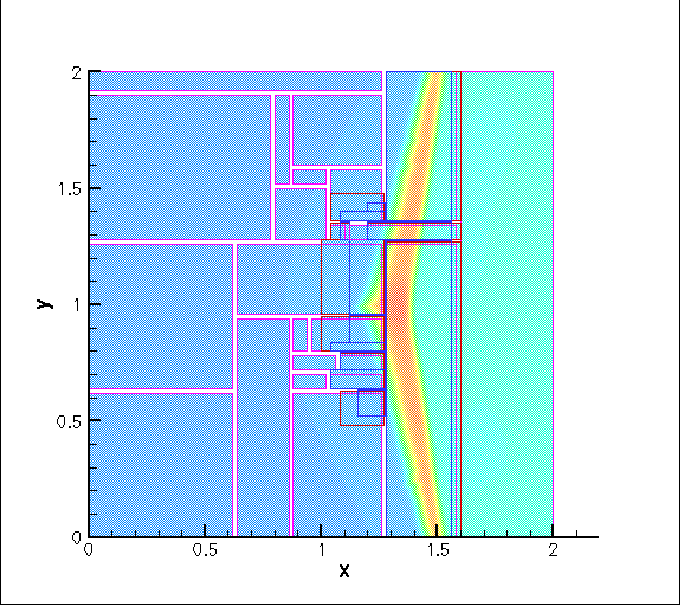Figure 2: Snapshot of the component application, as assembled for execution. We see three proxies (for AMRMesh, EFMFlux and States), as well as the TauMeasurement and Mastermind components to measure and record performance-related data.

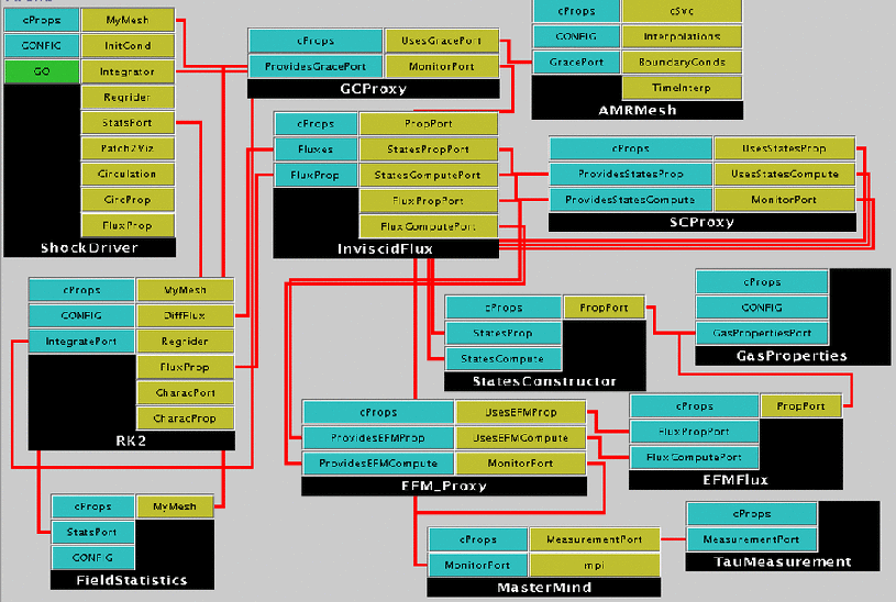Figure 3: Snapshot from a timing profile done with our infrastructure. We see that around 50% of the time is accounted for by g_proxy::compute(), sc_proxy::compute() and MPI_Waitsome(). The MPI call is invoked from AMRMesh. The two other methods are modeled as a part of the work reported here. Timings have been averaged over all the processors. The profile shows the inclusive time (total time spent in the methods and all subsequent method calls), exclusive time (time spent in the specific method less the time spent in subsequent instrumented methods), the number of times the method was invoked, and the average time per call to the method, irrespective of the data being passed into the method.

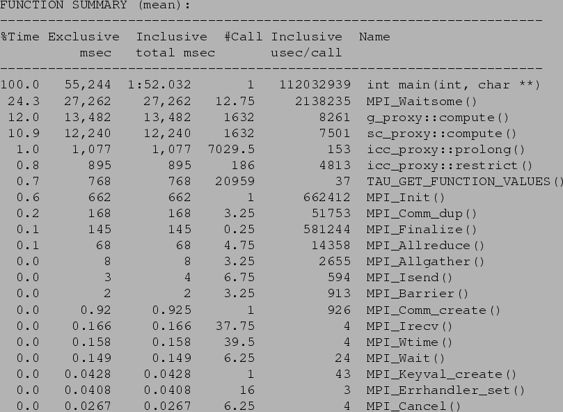Figure 4: Execution time for the States component. The States component is invoked in two modes, one which requires sequential and the other which requires strided access of arrays to calculate X- and Y- derivatives of a field. Both the times are plotted. The Y-derivative calculation (strided access) is expected to take longer for large arrays and this is seen in the spread of timings. For small array sizes, which are largely cache-resident, the two different modes of access do not result in a large difference in execution time. Array sizes are the actual number of elements in the array. The elements are double precision numbers. The different colors represent data from different processors (Proc $i$ in the legend) and similar trends are seen on all processors.

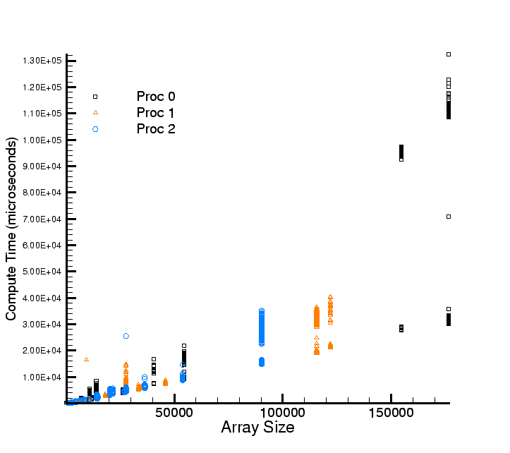Figure 5: Ratio of strided versus sequential access (calculation of Y- and X-derivatives, respectively) timings for States. We see that the ratio varies from around 1 for small array sizes to around 4 for the largest arrays considered here. Array sizes are the actual number of elements in the array. The elements are double precision numbers. Further, the ratios show variability which tend to increase with array size

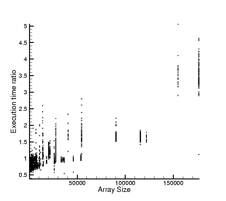Figure 6: Average execution time for States as a function of the array size. Since States has a dual mode of operation (sequential versus strided) and the mean includes both, the standard deviation of is rather large. The performance model is given in Eq. 1. The standard deviation, in blue, is plotted against the right Y-axis. All timings are in microseconds.

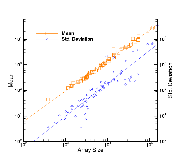Figure 7: Average execution time for GodunovFlux as a function of the array size. Since GodunovFlux has a dual mode of operation (sequential versus strided) and the mean includes both, the standard deviation of is rather large. The performance model is given in Eq. 1. The standard deviation, in blue, is plotted against the right Y-axis. All timings are in microseconds.

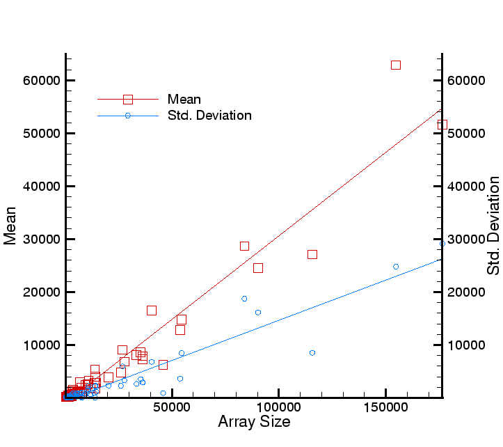Figure 8: Average execution time for EFMFlux as a function of the array size. Since EFMFlux has a dual mode of operation (sequential versus strided) and the mean includes both, the standard deviation of is rather large. The performance model is given in Eq. 1. The standard deviation, in blue, is plotted against the right Y-axis. All timings are in microseconds.

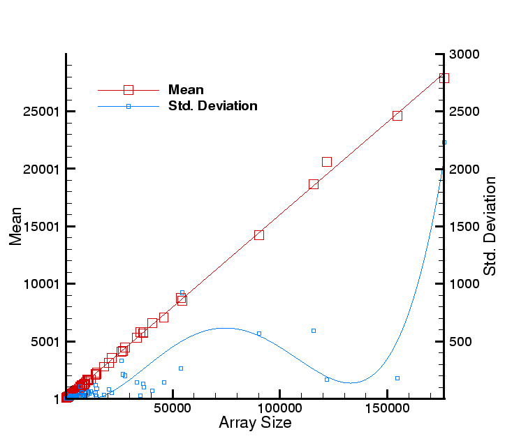Figure 9: Message passing time for different levels of the grid hierarchy for the 3 processors. We see a clustering of message passing times, especially for Levels 0 and 2. The grid hierarchy was subjected to a re-grid step during the simulation which resulted in a different domain decomposition and consequently message passing times. Inset : We plot the timings for all processors. Similar clustering is observed. All times are in microseconds.

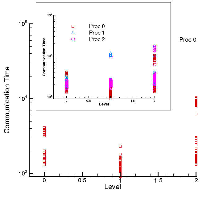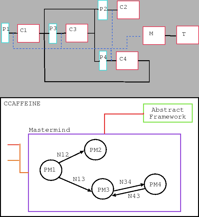
Figure 10: Above: A simple application composed of 4 components. C denotes a component, P denotes a proxy and M and T denote an instance of Mastermind and TauMeasurement components. The black lines denote port connection between components and the blue dashed lines are the proxy-to-Mastermind port connections which are only used for PMM. Below, it dual, constructed as a directed graph in the Mastermind, with edge weights corresponding to the number of invocations and the vertex weights being the compute and communication times determined from the performance models (PM$_i$) for component $i$. Only the port connections shown in black in the picture above are represented in the graph. The parent-child relationship is preserved to identify sub-graphs that do not contribute much to the execution time and thus can be neglected during component assembly optimization. The Mastermind is seen connected to CCAFFEINE via the AbstractFramework Port to enable dynamic replacement of sub-optimal components.