
-pdt=< dir > -mpiinc=< dir > -mpilib=< dir > options. To configure Hypre with TAU, use the -with-TAU=< dir > option. Once it is built, you can run any of the examples located in src/test directory to generate profile or trace data. Click here to see a script file the shows how to configure and build PDT, TAU, and Hypre in order to run together. It also illustrates how to execute one of the examples listed in /src/test/IJ_linear_solvers.sh in the Hypre distribution.
mpirun -np 4 IJ_linear_solvers -rhsrand -n 60 60 60 -P 2 2 1 -ruge -27pt. This example is similar to the examples used in the IJ_linear_solvers.sh file, but we increased the values of -n in order to increase the overall problem size with a longer overall execution time. 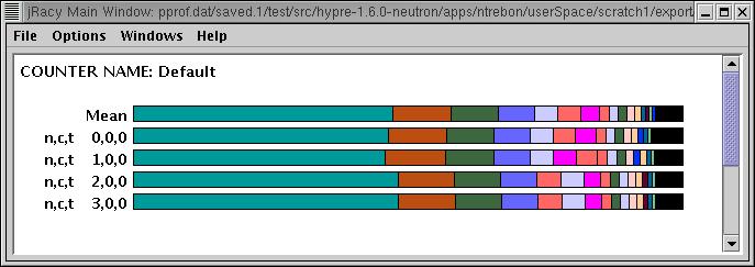
The above display (jracy) shows the profile of the hypre example. It was executed on four processors (node 0 through 3 in the main display). n,c,t 1,0,0 stands for node 1, context 0, thread 0. Color coded routines are seen in the Ledger window below.
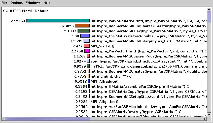
By clicking the first mouse button on a particular node (node 0, in this case) in the main racy window, the above picture shows the breakdown of time spent in routines for that particular node. The Options menu shows various sorting and display options.
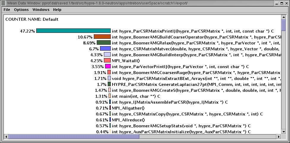
The above picture illustrates the mean percentage of execution inside each routine across all nodes.
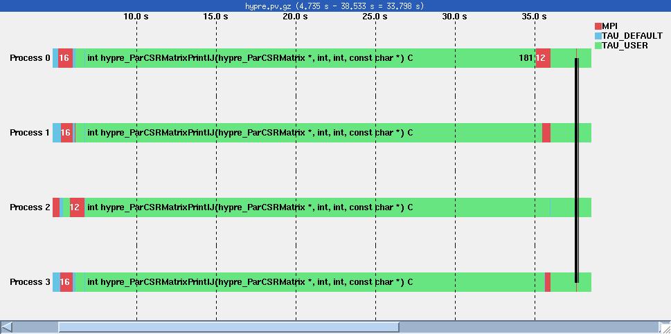
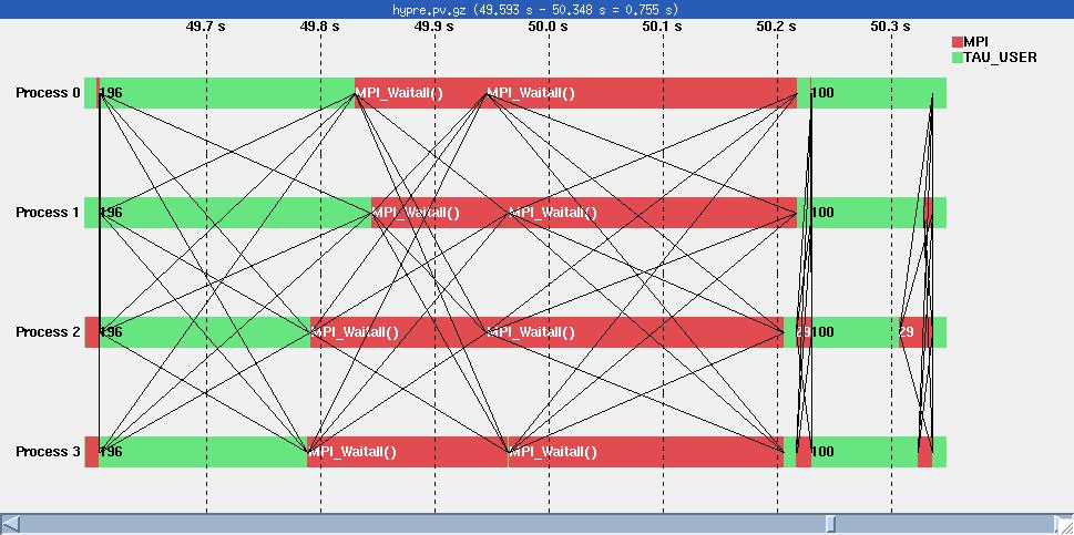
In the above figures, we see two timeline displays for two distinct ranges of the execution. Inter process communication is also seen as line segments. Vampir allows the user to zoom into a segment of the trace to examine the events on each node.
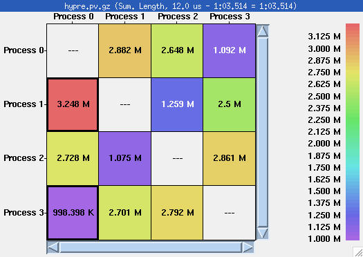
The above figure shows the communication matrix in Vampir. The extent of inter-process message communication is seen here.
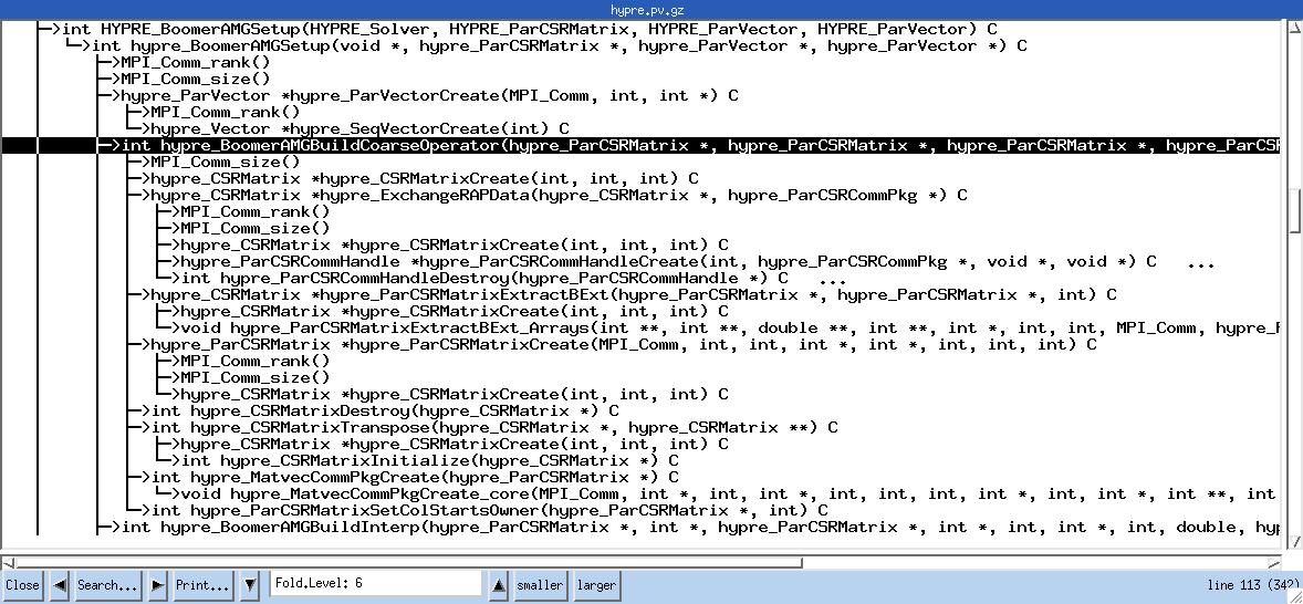
Tracing also preserves the dynamic calltree of a process. The calltree view on node 0 shows the time spent in various routines, as well as the number of times it was called and the calling order.