Scenario: One Send

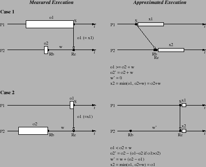
To begin, consider a single message sent between two processes, P1 and P2. Figure 2 shows the two possible cases, distinguishing which process has accumulated more overhead up until the time of the message communication. Execution time advances from left to right and shown on the timelines are send events ($S$) and receive events ($Rb$, receive begin; $Re$, receive end). The overhead on P1 is $o1$ and the overhead on P2 is $o2$. The overhead is shown as a blocked region immediately before the $S$ or $Rb$ events to easily see its size in the figure, but it is actually spread out across the preceding timeline where profiled events occur. Also designated is the waiting time ($w$) between $Rb$ and $Re$, assuming waiting time can be measured by the profiling system.

Figure 2: Two-Process, One-Send - Models and Analysis

Case 1 occurs when P1's overhead is greater than or equal to P2's overhead plus the waiting time ( $o1 \geq o2 + w$). A rational reconstruction of the approximated execution determines that P2 would not have waited for the message (i.e., $S$ would occur earlier than $Rb$). Hence, the approximated waiting time (designated as $w'$) should be zero, as seen in the approximated execution timeline. Of course, the problem is that P2 has already waited in the measured execution for the message to be received. In order for P2 to know P1's message would have arrived earlier, P1 must communicate this information. Clearly, the information is exactly the value $o1$, P1's overhead. This is indicated in the figure by tagging the message communication arrow with this value.

With P1's overhead information, P2 can determine what to do about the waiting time. The waiting time has already been measured and must be correctly accounted. If the approximated waiting is adjusted to zero, where should the elapsed time represented by $w$ go? If the profiling overhead is to be correctly compensated, the measured waiting time must be attributed to P2's approximated overhead ($o2' = o2 + w$)! This is interesting because it shows how, even in a very simple case, the naive overhead compensation can lead to errors without conveyance of delay information between sender and receiver. It is also important to note that $Rb$ cannot be moved back any further in the approximated execution. This suggests that the only correction we can ever make in the receiver is in respect to waiting time.

The overhead value sent by P1 with the message conveys to P2 the information ``this message was delayed being sent by $o1$ amount of time'' or ``this message would have been sent $o1$ time units earlier.'' We contend that this is exactly the information needed by P2 to correctly adjust its profiling metrics (i.e., compensate for overhead in parallel execution). We refer to the value sent by P1 as delay and will assign the designator $x$ to represent its modeling and analysis that follows. For instance, P1's delay is given by $x1$. In this case, $x1=o1$, but it is not always true that delay will be equal to accumulated overhead, as we will see. Now an interesting question arises. How much earlier would future events on process 2 occur in the approximated execution after the message from P1 has been received? In general, each process will maintain a delay value ($xi$ for process Pi) for it to include in its next send message to tell the receiving process how much earlier the message would have been sent. In the approximated execution, for denotational purposes, we show the $x1$ and $x2$ values for P1 and P2 as shaded regions after the last events, $S$ and $Re$, respectively. We also show an expression for the calculation of $x2$ for this case.

Moving on to the second case, the overhead and waiting time in P2 is greater than what P1 reports (i.e., $o1 < o2 + w$). Rationally, this means that $S$ happens after $Rb$ in the approximated execution. What is the effect on $w'$, the approximated waiting time? Interesting, $w'$ can increase or decrease, depending on the relation of $o1$ to $o2$. (Remember, $o1$ is the same as $x1$ in these cases.) However, the occurrence of $Re$ is certainly dependent on $S$ and, thus, $x2$ will be entirely determined by (and, in fact, equal to) $x1$.

If this was all the two processes did, the models and analysis expressions would be all we need. Unfortunately, life is not so simple. Let us add in a bit more complexity.