Scenario: Two Sends

To gain a better understanding of this concept of a process carrying forward a delay quantity ($x$) indicating how much earlier the next future send event would occur, we look at the scenario of sending two messages. This is shown in Figure 3. There are four cases to consider. In each case, we show the analysis of the first message following the modeling methods demonstrated above. Then we consider the second message. Notice the inclusion of additional profiling overheads in the two processes after the first message ($o1a$ and $o2a$) as well as a second waiting term ($y$) in P2.

Figure 3: Two-Process, Two-Send - Models and Analysis (Case: 1, 2)

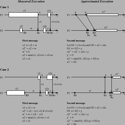
Consider Case 1. The first message is approximated exactly as in Case 1 of the single send model. P1's second send event is easily approximated by subtracting the accumulated overheads. P1's delay is exactly this accumulated overhead ($o1+o1a$) and this information should be sent to P2, as shown. P2's second receive begins a known amount of time after the first receive completes. However, to correctly compensate for profiling overhead, P2 must be able to determine the relative timing of the second $Rb$ event and the second $S$ event.

Figure 4: Two-Process, Two-Send - Models and Analysis (Case: 3, 4)

With the $x2$ delay calculation from the first receive, P2 has all the information it needs. By comparing the value $o1+o1a$ sent with the second message to $x2$ plus any additional overhead and waiting time on P2 ($o2a+y$), we can determine if the send event or the receive event occurred earlier in the approximated execution. The second message analysis introduces two new variables ($O1$ and $O2$), to bring out the similarities in the expressions for the One Send models. As seen, P2 should never wait in its approximated execution. Thus, its immediate future events would occur earlier by an amount based solely on its accumulated overhead and the waiting time it erroneously incurred. This analysis is successfully captured with the expressions shown. Interestingly, these expressions have a strong similarity to the One Send cases.

Does this similarity continue to hold for Case 2? Here, we have the alternate first message case (i.e., $Rb$ occurs before $S$ in the approximated execution), and the one send analysis determines the value of $x2$. However, our rational reconstruction leads to second message equations that are exactly the same as in Case 1. That is, after the effects of the first message have been approximated, we see that P2 would not have waited for the second message, just as in Case 1.

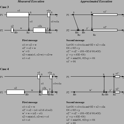
The similarity in the form of the equations suggest that it may be possible to handle the overhead compensation on a message-by-message basis. We argue that the $x$ delay values maintained by a process are the key. This is evidenced in the last two cases for the Two Sends scenario shown in Figure 4. These two cases differ from the first two in respect to the outcome of the conditional test between $O1$ and $O2+y$. Here we consider two situations where waiting will occur in the second message approximation. Following the expression pattern for processing this case in the One Send scenario, the equations result in a correct updating of the overhead and waiting values. In addition, the values of $x1'$ and $x2'$ are consistently calculated.