ParaProf - User’s Manual
Introduction
ParaProf is a portable, scalable performance analysis tool included with the TAU distribution.
|
ParaProf requires Oracle / Sun’s Java 1.5 Runtime Environment for basic functionality. Java JOGL (included) is required for 3d visualization and image export. Additionally, OpenGL is required for 3d visualization. |
|
Most windows in ParaProf can export bitmap (png/jpg) and vector (svg/eps) images to disk (png/jpg) or print directly to a printer. This are available through the File menu. |
Using ParaProf from the command line
ParaProf is a java program that is run from the supplied paraprof script ( paraprof.bat for windows binary release).
% paraprof --help
Usage: paraprof [options] <files/directory>

Options:

  -f, --filetype <filetype>       Specify type of performance data, options are:
                                    profiles (default), pprof, dynaprof, mpip,
                                    gprof, psrun, hpm, packed, cube, hpc, ompp
                                    snap, perixml, gptl, ipm, google
  --range a-b:c                   Load only profiles from the given range(s) of processes
                                    Seperate individual ids or dash-defined ranges with colons
  -h, --help                      Display this help message

The following options will run only from the console (no GUI will launch):

  --merge <file.gz>               Merges snapshot profiles
  --pack <file>                   Pack the data into packed (.ppk) format
  --dump                          Dump profile data to TAU profile format
  --dumprank <rank>               Dump profile data for <rank> to TAU profile format
  -v, --dumpsummary               Dump derived statistical data to TAU profile format
  --overwrite                     Allow overwriting of profiles
  -o, --oss                       Print profile data in OSS style text output
  -q, --dumpmpisummary            Print high level time and communication summary
  -d, --metadump                  Print profile metadata (works with --dumpmpisummary)
  -x, --suppressmetrics           Exclude child calls and exclusive time from --dumpmpisummary
  -s, --summary                   Print only summary statistics
                                    (only applies to OSS output)

Notes:
  For the TAU profiles type, you can specify either a specific set of profile
files on the commandline, or you can specify a directory (by default the current
directory).  The specified directory will be searched for profile.*.*.* files,
or, in the case of multiple counters, directories named MULTI_* containing
profile data.
Supported Formats
ParaProf can load profile date from many sources. The types currently supported are:
TAU Profiles (profiles) - Output from the TAU measurement library, these files generally take the form of profile.X.X.X , one for each node/context/thread combination. When multiple counters are used, each metric is located in a directory prefixed with "MULTI". To launch ParaProf with all the metrics, simply launch it from the root of the MULTI directories.
ParaProf Packed Format (ppk) - Export format supported by PerfDMF/ParaProf. Typically .ppk.
TAU Merged Profiles (snap) - Merged and snapshot profile format supported by TAU. Typically tauprofile.xml.
TAU pprof (pprof) - Dump Output from TAU’s pprof -d . Provided for backward compatibility only.
DynaProf (dynaprof) - Output From DynaProf’s wallclock and papi probes.
mpiP (mpip) - Output from mpiP.
gprof (gprof) - Output from gprof, see also the --fixnames option.
PerfSuite (psrun) - Output from PerfSuite psrun files.
HPM Toolkit (hpm) - Output from IBM’s HPM Toolkit.
Cube (cube) - Output from Kojak Expert tool for use with Cube.
Cube3 (cube3) - Output from Kojak Expert tool for use with Cube3 and Cube4.
HPCToolkit (hpc) - XML data from hpcquick. Typically, the user runs hpcrun, then hpcquick on the resulting binary file.
OpenMP Profiler (ompp) - CSV format from the ompP OpenMP Profiler (http://www.ompp-tool.com). The user must use OMPP_OUTFORMAT=CVS.
PERI XML (perixml) - Output from the PERI data exchange format.
General Purpose Timing Library (gptl) - Output from the General Purpose Timing Library.
Paraver (paraver) - 2D output from the Paraver trace analysis tool from BSC.
IPM (ipm) - Integrated Performance Monitoring format, from NERSC.
Google (google) - Google Profiles.
Command line options
In addition to specifying the profile format, the user can also specify the following options
-
--fixnames - Use the fixnames option for gprof. When C and Fortran code are mixed, the C routines have to be mapped to either .function or function_. Strip the leading period or trailing underscore, if it is there.
-
--pack <file> - Rather than load the data and launch the GUI, pack the data into the specified file.
-
--dump - Rather than load the data and launch the GUI, dump the data to TAU Profiles. This can be used to convert supported formats to TAU Profiles.
-
--oss - Outputs profile data in OSS Style. Example:
-------------------------------------------------------------------------------
Thread: n,c,t 0,0,0
-------------------------------------------------------------------------------
 excl.secs  excl.%   cum.%    PAPI_TOT_CYC     PAPI_FP_OPS     calls  function
     0.005   56.0%   56.0%        13475345         4194518         1  foo
     0.003   40.1%   96.1%         9682185         4205367         1  bar
         0    3.6%   99.7%          223173           17445         1  baz
   2.2E-05    0.3%  100.0%           14663             206         1  main
-
--summary - Output only summary information for OSS style output.
Views and Sub-Views
In the past, PerfDMF used a hierarchy of Applications and Experiments to organize Trials. This approach was too rigid, so in TAUdb, trials are organized by dynamic Views. Views are lists of Trials that share a given metadata value. For example, a View could contain all the Trials where the total number of threads is less than 16. Views can also have Sub-Views. For example, it might be useful to have a View of all Trials from a certain machine and then Sub-Views for each executable ran on that machine. Trials can belong to any number of VIews and Sub-Views and new Trials loaded to the database will be sorted into Views automatically.
To Create a (Sub-)Views
Launch ParaProf and Right click on a database or an existing View and select "Add View" or "Add Sub-View."

This will launch the View Creator window.
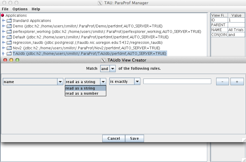
Here you can create the rule(s) for which Trials appear in this new View. At the top you can choose to match all of the rules ("and") or to match any of the rules. The "-" or "=" buttons will remove the current rule or add a new one. The first drop down box chooses which metadata field to use. The second box chooses whether the field should be read as a string or a number. Depending on whether it is read as a string or a number, the fourth box will give options on how to compare the metadata field. So to create a View for all trials that have less than 16 threads, select total_threads, read as a string, is less than, 16. Then click Save and give the View a name.
The 'Edit' context menu option on an existing view will allow you to view and alter the view’s criteria in the same interface.
Profile Data Management
ParaProf uses PerfDMF to manage profile data. This enables it to read the various profile formats as well as store and retrieve them from a database.
ParaProf Manager Window
Upon launching ParaProf, the user is greeted with the ParaProf Manager Window.
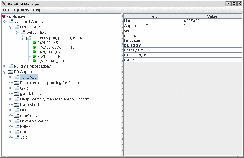
This window is used to manage profile data. The user can upload/download profile data, edit meta-data, launch visual displays, export data, derive new metrics, etc.
Loading Profiles
To load profile data, select File→Open, or right click on the Application’s tree and select "Add Trial".
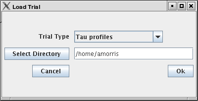
Select the type of data from the "Trial Type" drop-down box. For TAU Profiles, select a directory, for other types, files.
Database Interaction
Database interaction is done through the tree view of the ParaProf Manager Window. Applications expand to Experiments, Experiments to Trials, and Trials are loaded directly into ParaProf just as if they were read off disk. Additionally, the meta-data associated with each element is show on the right, as in ParaProf Manager Window . A trial can be exported by right clicking on it and selecting "Export as Packed Profile".
New trials can be uploaded to the database by either right-clicking on an entity in the database and selecting "Add Trial", or by right-clicking on an Application/Experiment/Trial hierarchy from the "Standard Applications" and selecting "Upload Application/Experiment/Trial to DB".
Creating Derived Metrics
ParaProf can created derived metrics using the Derived Metric Panel , available from the Options menu of the ParaProf Manager Window.
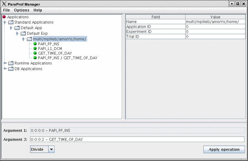
In Creating Derived Metrics , we have just divided Floating Point Instructions by Wall-clock time, creating FLOPS (Floating Point Operations per Second). The 2nd argument is a user editable text-box and can be filled in with scalar values by using the keyword 'val' (e.g. "val 1.5").
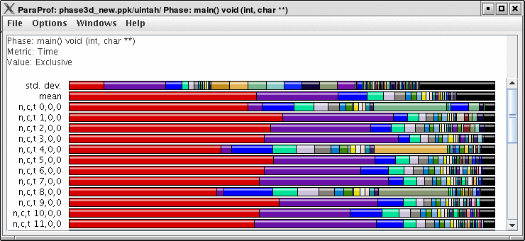
Main Data Window
Upon loading a profile, or double-clicking on a metric, the Main Data Window will be displayed.
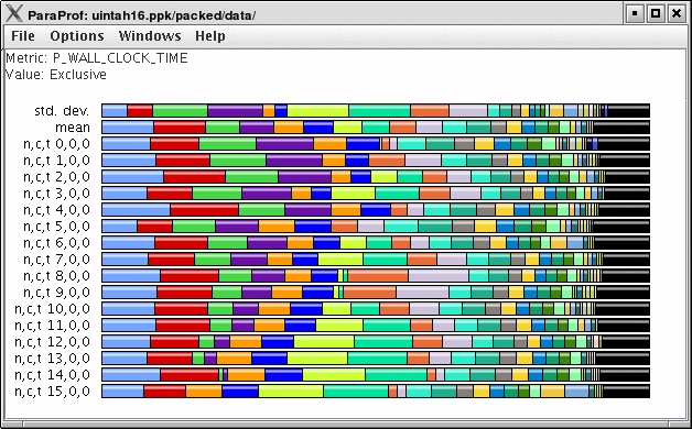
This window shows each thread as well as statistics as a combined bar graph. Each function is represented by a different color (though possibly cycled). From anywhere in ParaProf, you can right-click on objects representing threads or functions to launch displays associated with those objects. For example, in Main Data Window , right click on the text n,c,t, 8,0,0 to launch thread based displays for node 8.

You may also turn off the stacking of bars so that individual functions can be compared across threads in a global display.
3-D Visualization
ParaProf displays massive parallel profiles through the use of OpenGL hardware acceleration through the 3D Visualization window. Each window is fully configurable with rotation, translation, and zooming capabilities. Rotation is accomplished by holding the left mouse button down and dragging the mouse. Translation is done likewise with the right mouse button. Zooming is done with the mousewheel and the + and - keyboard buttons.
Triangle Mesh Plot

This visualization method shows two metrics for all functions, all threads. The height represents one chosen metric, and the color, another. These are selected from the drop-down boxes on the right.
To pinpoint a specific value in the plot, move the Function and Thread sliders to cycle through the available functions/threads. The values for the two metrics, in this case for MPI_Recv() on Node 351 , the value is 14.37 seconds.
3-D Bar Plot

This visualization method is similar to the triangle mesh plot. It simply displays the data using 3d bars instead of a mesh. The controls works the same. Note that in 3-D Mesh Plot the transparency option is selected, which changes the way in which the selection model operates.
3-D Scatter Plot

This visualization method plots the value of each thread along up to 4 axes. Each axis represents a different function and metric. This view allows you to discern clustering of values and relationships between functions across threads.
Select functions using the button for each dimension, then select a metric. A single function across 4 metrics could be used, for example.
3-D Topology Plot

In this visualization, you can either define the layout with a MESP topology definition file or you can fill a rectangular prism of user-defined volume with rank-points in order of rank. For more information, please see the etc/topology directory for additional details on MESP topology definitions.
If the loaded profile is a cube file or a profile from a BGB, then this visualizations groups the threads in two or three dimensional space using topology information supplied by the profile.
When topology metadata is available a trial-specific topological layout may be visualized by selecting Windows→gt;3D Visualization and selecting Topology Plot on the visualization pane.
The layout tab allows control of the layout and display of visualized cores/processes.
Minimum/Maximum Visible (restricts display of nodes with measured values above/below the selected levels). Lock Range causes the sliders to move in unison.
The X/Y/Z Axis sliders allow selection of planes, lines and individual points in the topology for examination of specific values in the display, listed in the Avg. Color Value field.
The topology selection dropdown box allows selection of either trial-specific topologies contained in the metadata, mapped topologies stored in an external file or a custom topology defined by the size of the prism containing the visualized cores. The … button allows selection of a custom topology mapping file while the map button allows selection of a map file (see <tau2>/etc/topology/README.cray_map for more information on generating map files).
If a Custom is selected the dimensions of the rectangular prism containing the cores are defined by the X/Y/Z axis control widgets.
The Events tab controls which events are used to define the color values and positions of cores/processes in the display. For trail-specific and Custom topologies only event3(Color) can be changed. For topologies loaded in MESP definition files all four events may be used in calculation of the topology layout. In either case, interval, atomic or metadata values may be used to color or position points in the display.

Thread Based Displays
ParaProf displays several windows that show data for one thread of execution. In addition to per thread values, the users may also select mean or standard deviation as the "thread" to display. In this mode, the mean or standard deviation of the values across the threads will be used as the value.
Thread Bar Graph

This display graphs each function on a particular thread for comparison. The metric, units, and sort order can be changed from the Options menu.
Thread Statistics Text Window
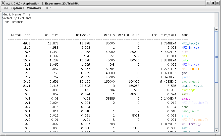
This display shows a pprof style text view of the data.
Thread Statistics Table
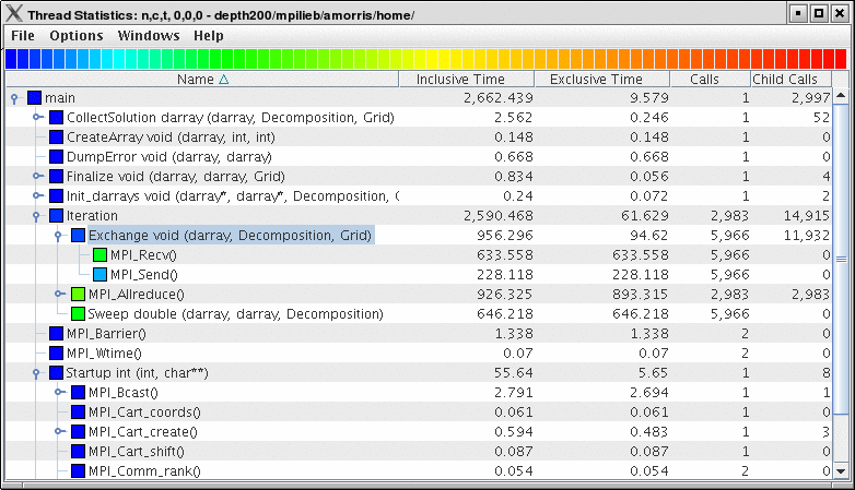
This display shows the callpath data in a table. Each callpath can be traced from root to leaf by opening each node in the tree view. A colorscale immediately draws attention to "hot spots", areas that contain highest values.


The display can be used in one of two ways, in "inclusive/exclusive" mode, both the inclusive and exclusive values are shown for each path, see Thread Statistics Table, inclusive and exclusive for an example.
When this option is off, the inclusive value for a node is show when it is closed, and the exclusive value is shown when it is open. This allows the user to more easily see where the time is spent since the total time for the application will always be represented in one column. See Thread Statistics Table and Thread Statistics Table for examples. This display also functions as a regular statistics table without callpath data. The data can be sorted by columns by clicking on the column heading. When multiple metrics are available, you can add and remove columns for the display using the menu.
Call Graph Window
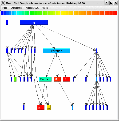
This display shows callpath data in a graph using two metrics, one determines the width, the other the color. The full name of the function as well as the two values (color and width) are displayed in a tooltip when hovering over a box. By clicking on a box, the actual ancestors and descendants for that function and their paths (arrows) will be highlighted with blue. This allows you to see which functions are called by which other functions since the interplay of multiple paths may obscure it.
Thread Call Path Relations Window

This display shows callpath data in a gprof style view. Each function is shown with its immediate parents. For example, Thread Call Path Relations Window shows that MPI_Recv() is call from two places for a total of 9.052 seconds. Most of that time comes from the 30 calls when MPI_Recv() is called by MPIScheduler::postMPIRecvs() . The other 60 calls do not amount to much time.
User Event Statistics Window

This display shows a pprof style text view of the user event data. Right clicking on a User Event will give you the option to open a Bar Graph for that particular User Event across all threads. See User Event Bar Graph
User Event Thread Bar Chart

This display shows a particular thread’s user defined event statistics as a bar chart. This is the same data from the User Event Statistics Window , in graphical form.
Function Based Displays
ParaProf has two displays for showing a single function across all threads of execution. This chapter describes the Function Bar Graph Window and the Function Histogram Window.
Function Bar Graph

This display graphs the values that the particular function had for each thread along with the mean and standard deviation across the threads. You may also change the units and metric displayed from the Options menu.
Function Histogram

This display shows a histogram of each thread’s value for the given function. Hover the mouse over a given bar to see the range minimum and maximum and how many threads fell into that range. You may also change the units and metric displayed from the Options menu.
You may also dynamically change how many bins are used (1-100) in the histogram. This option is available from the Options menu. Changing the number of bins can dramatically change the shape of the histogram, play around with it to get a feel for the true distribution of the data.
Phase Based Displays
When a profile contains phase data, ParaProf will automatically run in phase mode. Most displays will show data for a particular phase. This phase will be displayed in teh top left corner in the meta data panel.
Using Phase Based Displays
The initial window will default to top level phase, usually main
To access other phases, either right click on the phase and select, "Open Profile for this Phase", or go to the Phase Ledger and select it there.

ParaProf can also display a particular function’s value across all of the phases. To do so, right click on a function and select, "Show Function Data over Phases".

Because Phase information is implemented as callpaths, many of the callpath displays will show phase data as well. For example, the Call Path Text Window is useful for showing how functions behave across phases.
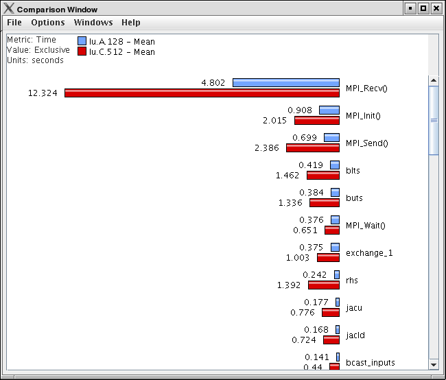
Comparative Analysis
ParaProf can perform cross-thread and cross-trial anaylsis. In this way, you can compare two or more trials and/or threads in a single display.
Using Comparitive Analysis
Comparative analysis in ParaProf is based on individual threads of execution. There is a maximum of one Comparison window for a given ParaProf session. To add threads to the window, right click on them and select "Add Thread to Comparison Window". The Comparison Window will pop up with the thread selected. Note that "mean" and "std. dev." are considered threads for this any most other purposes.

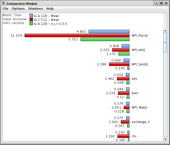
Add additional threads, from any trial, by the same means.
Miscellaneous Displays
User Event Bar Graph
In addition to displaying the text statistics for User Defined Events, ParaProf can also graph a particular User Event across all threads.

This display graphs the value that the particular user event had for each thread.
Ledgers
ParaProf has three ledgers that show the functions, groups, and user events.
Function Ledger

The function ledger shows each function along with its current color. As with other displays showing functions, you may right-click on a function to launch other function-specific displays.
Group Ledger

The group ledger shows each group along with its current color. This ledger is especially important because it gives you the ability to mask all of the other displays based on group membership. For example, you can right-click on the MPI group and select "Show This Group Only" and all of the windows will now mask to only those functions which are members of the MPI group. You may also mask by the inverse by selecting "Show All Groups Except This One" to mask out a particular group.

Selective Instrumentation File Generator
ParaProf can also help you refine your program performance by excluding some functions from instrumentation. You can select rules to determine which function get excluded; both rules must be true for a given function to be excluded. Below each function that will be excluded based on these rules are listed.

|
Only the functions profilied in ParaProf can be excluded. If you had previously setup selective instrumentation for this application the functions that where previously excluded will not longer be excluded. |
Preferences
Preferences are modified from the ParaProf Preferences Window, launched from the File menu. Preferences are saved between sessions in the .ParaProf/ParaProf.prefs
Preferences Window
In addition to displaying the text statistics for User Defined Events, ParaProf can also graph a particular User Event across all threads.

The preferences window allows the user to modify the behavior and display style of ParaProf’s windows. The font size affects bar height, a sample display is shown in the upper-right.
The Window defaults section will determine the initial settings for new windows. You may change the initial units selection and whether you want values displayed as percentages or as raw values.
The Settings section controls the following
-
Show Path Title in Reverse - Path title will normally be shown in normal order (/home/amorris/data/etc). They can be reverse using this option (etc/data/amorris/home). This only affects loaded trials and the titlebars of new windows.
-
Reverse Call Paths - This option will immediately change the display of all callpath functions between
Root ⇒ LeafandLeaf ⇐ Root. -
Statistics Computation - Turning this option on causes the mean computation to take the sum of value for a function across all threads and divide it by the total number of threads. With this option off the sum will only be divided by the number of threads that actively participated in the sum. This way the user can control whether or not threads which do not call a particular function are consider as a
0in the computation of statistics. -
Generate Reverse Calltree Data - This option will enable the generation of reverse callpath data necessary for the reverse callpath option of the statistics tree-table window.
-
Show Source Locations - This option will enable the display of source code locations in event names.
Default Colors
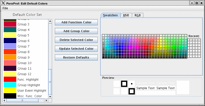
The default color editor changes how colors are distributed to functions whose color has not been specifically assigned. It is accessible from the File menu of the Preferences Window.
Color Map
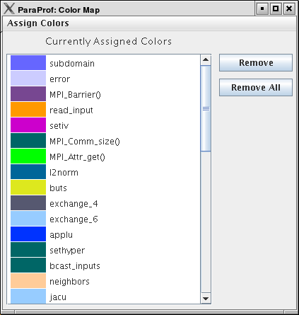
The color map shows specifically assigned colors. These values are used across all trials loaded so that the user can identify a particular function across multiple trials. In order to map an entire trial’s function set, Select "Assign Defaults from →" and select a loaded trial.
Individual functions can be assigned a particular color by clicking on them in any of the other ParaProf Windows.